Visualize and analyse IMDB ratings with R (part 2)

Does popularity of a movie impact my rating?

Some movies are very mainstream, other are more niche or an “acquired” taste. The popularity of a movie can be determined in IMDB by the number of reviews a movie has received. Let’s first see how the number of IMDB reviews relates to the average IMDB rating. We can do that by building a sctaterplot.

theme_data <- theme_light(base_size = 13) + theme(plot.margin=unit(c(0.5,1,1.5,1.2),"cm")) 
color_bar <- "#999999"
color_fill <- "#5c85d6"
#spread of movie release decades
ggplot(data_imdb, aes(x = imdb_ratings, y = imdb_rating)) +
  geom_point() +
  #scale_x_discrete(limit = c(1930, 1940, 1950, 1960, 1970, 1980, 1990, 2000, 2010)) + 
  scale_y_discrete(limit = c(3:10)) + 
  ylab("IMDB average rating") +
  xlab("Number of IMDB ratings") +   
  theme_data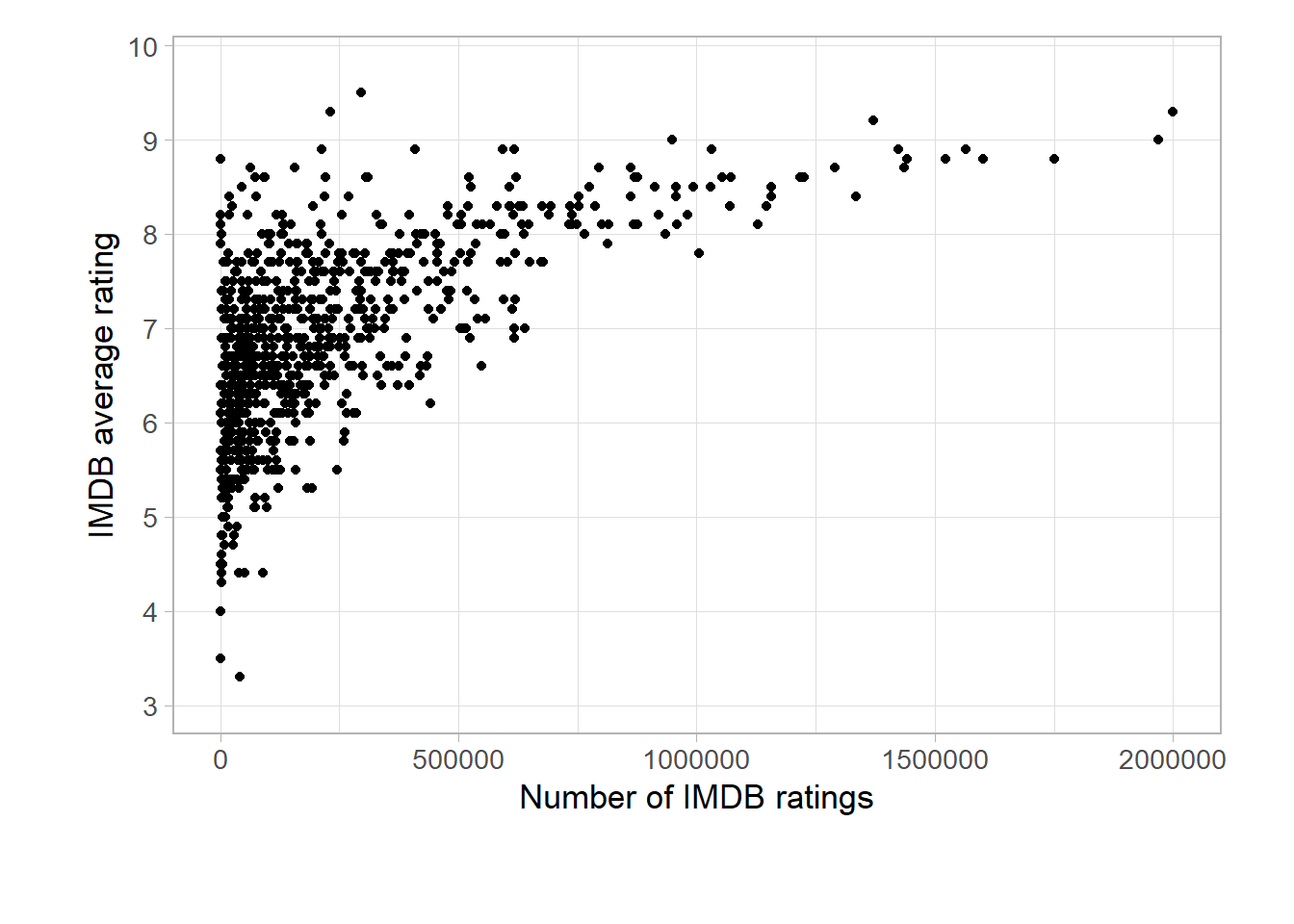

In this scatterplot you can see that most of the movies are clustered around a low number of reviews and are receiving average ratings between 6 and 7. It’s interesting to see that the movies with most IMDB ratings are all highly rated. Let’s check out which movies these are.

head(arrange(data_imdb[,c("title", "imdb_ratings", "imdb_rating")],desc(imdb_ratings)),10)

##                                                title imdb_ratings imdb_rating
## 1                           The Shawshank Redemption      2000322         9.3
## 2                                    The Dark Knight      1969523         9.0
## 3                                          Inception      1750193         8.8
## 4                                         Fight Club      1600985         8.8
## 5                                       Pulp Fiction      1565763         8.9
## 6                                       Forrest Gump      1522234         8.8
## 7  The Lord of the Rings: The Fellowship of the Ring      1441273         8.8
## 8                                         The Matrix      1435239         8.7
## 9      The Lord of the Rings: The Return of the King      1424377         8.9
## 10                                     The Godfather      1370383         9.2

So Shawshank Redemption and Dark Knight are the most reviewed movies I have rated myself. And they are both highly rated.

cor(as.numeric(data_imdb$imdb_ratings), as.numeric(data_imdb$myRating))

## [1] 0.4478298

My favorite actors

I always think I know which actors I like and put their movies on the top of my watchlist. Let’s check out if I actually rate the movies my favorite actors with the highest scores too.

For each movies I rate, there are a maximum of 15 actors added to the dataset. I have added them all to one column, pipe separated. I will use the data.table and stringr package to split the data in the cast column and learn more about the actors in the movies I reviewed. I will create a new dataframe with a count of the the actors (unique_actor_count) and find out how many actors are in this dataframe (unique_actors). After that, I will create a new dataframe with my top 10 most watched actors and visualise it in a barchart for easy interpretation.

library('data.table')
library('stringr')
as.character(data_imdb$imdb_cast) -> data_imdb$imdb_cast
data.frame(table(unlist(strsplit(data_imdb$imdb_cast, "[|]")))) -> unique_actor_count

nrow(unique_actor_count) -> unique_actors
head(arrange(unique_actor_count,desc(Freq)),10) -> unique_actor_count_top10

ggplot(data = unique_actor_count_top10, aes(x = Var1, y = Freq)) +
  geom_bar(stat = "identity", fill=color_fill, color = color_bar)+
  coord_flip() +
  geom_text(aes(label = Freq), position=position_dodge(width=1), hjust = -0.5) + 
  theme(axis.text.x = element_text(angle = 90, hjust = 1)) +
  ylab("Number of movies watched featuring actor") +
  xlab("") +
  theme_data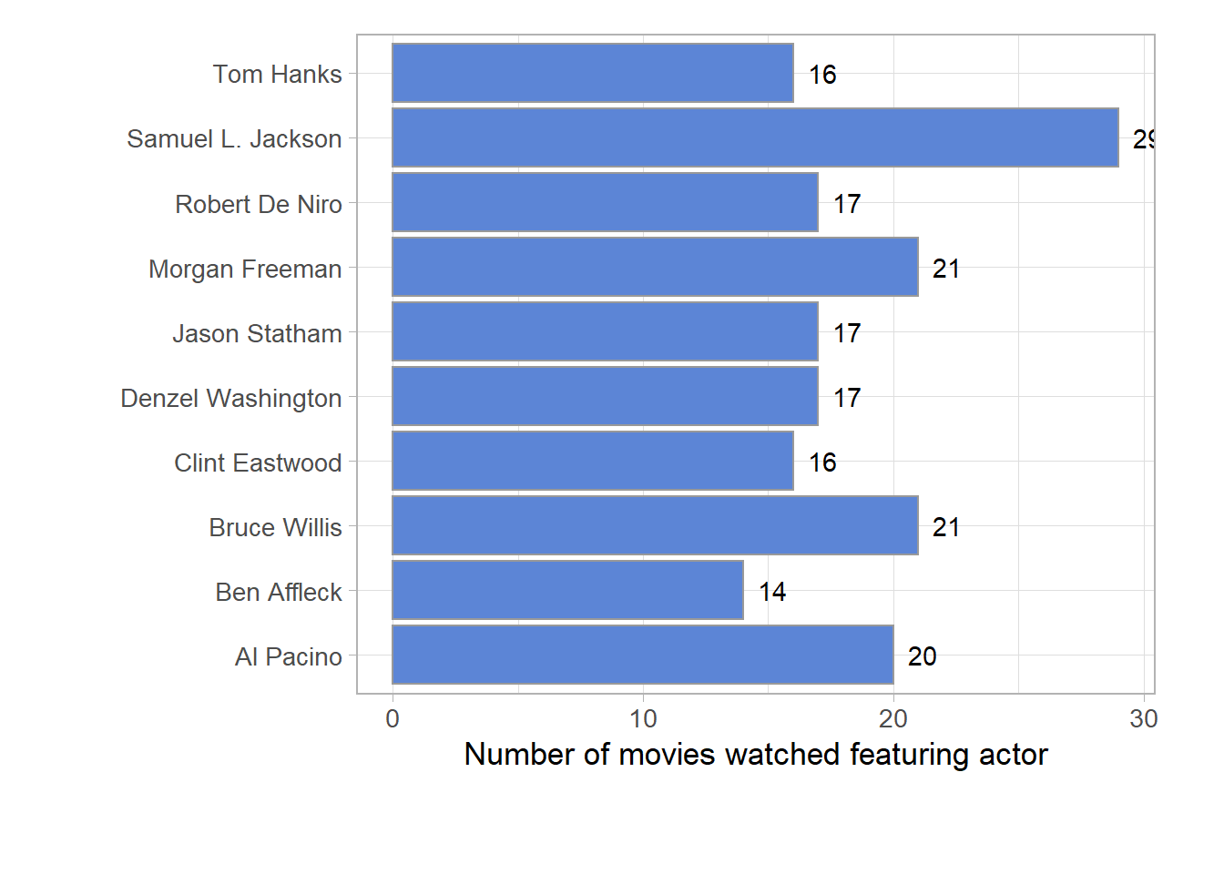

It turns out more than 8000 actors have made it to my dataframe and the one I have viewed more than others was Samuel L. Jackson. I’m surprised to see only male actors made it to my top 10. Not sure how that happened…

library('ggrepel')
head(arrange(unique_actor_count,desc(Freq)),100) -> unique_actor_count_top100
unique_actor_count_top100$Var1 -> actor_group
df_mean_actor <- data.frame()
for(v in actor_group){
  data_imdb %>%
    filter(str_detect(imdb_cast, v)) %>%
    select(myRating) -> df9
  round(mean(df9$myRating),2) ->mean_actor
  df10 <- data.table("actor" = v, "mean" = mean_actor)
  df_mean_actor<-rbind(df_mean_actor,df10)
}

actor_overview = merge(unique_actor_count_top100, df_mean_actor, by.x=c("Var1"), by.y=c("actor"))

ggplot(data = actor_overview, aes(x = mean, y = Freq)) +
  geom_point() +
  geom_text_repel(aes(label=ifelse(mean>7.5,as.character(Var1),'')), color = "forestgreen", box.padding = unit(0.8, "lines")) +
  geom_text_repel(aes(label=ifelse(mean<5.8,as.character(Var1),'')), color = "red", box.padding = unit(2.2, "lines")) +
  ylab("Number of movies watched featuring actor") +
  xlab("Average rating") +
  theme_data

My favorite movie genres

Just like my favorite actors, I can also learn more about favorite genres. The data is setup in the same way, so for now I will go straight to the visualisations.

as.character(data_imdb$imdb_genres) -> data_imdb$imdb_genres
data.frame(table(unlist(strsplit(data_imdb$imdb_genres, "[|]")))) -> unique_genres_count
c("Addcontentadvisoryforparents", "MPAA", "Seeallcertifications", "Viewcontentadvisory") -> genre_dirt
filter(unique_genres_count, !grepl(paste(genre_dirt, collapse="|"), Var1)) -> unique_genres_count
nrow(unique_genres_count)

## [1] 22

Just like actors, it is possible for a movie to have multiple genres. I have made them unique and can now see that I only have 22 genres in the dataset.

Let’s see what the average rating is per genre and the number of movies I have watched by genre.

head(arrange(unique_genres_count,desc(Freq)),10) -> unique_genres_count_top10

unique_genres_count$Var1 -> genre_group

df_mean_genre <- data.frame()
for(v in genre_group){
  data_imdb %>%
    filter(str_detect(imdb_genres, v)) %>%
    select(myRating) -> df7
    round(mean(df7$myRating),2) ->mean_genre
    df8 <- data.table("genre" = v, "mean" = mean_genre)
    df_mean_genre<-rbind(df_mean_genre,df8)
}

genre_overview = merge(unique_genres_count, df_mean_genre, by.x=c("Var1"), by.y=c("genre"))

ggplot(data = genre_overview, aes(x = Var1, y = mean, fill = Freq)) +
  geom_bar(stat = "identity")+
  geom_text(aes(label = mean), size = 3, position=position_dodge(width=1), vjust = -1) + 
  scale_y_continuous(expand = c(0, 0),breaks = seq(0, 10, 1), limits = c(0,8)) +  
  ylab("Average rating") +
  xlab("Genre") +
  theme_data +  
  theme(axis.text.x = element_text(angle = 90, hjust = 1))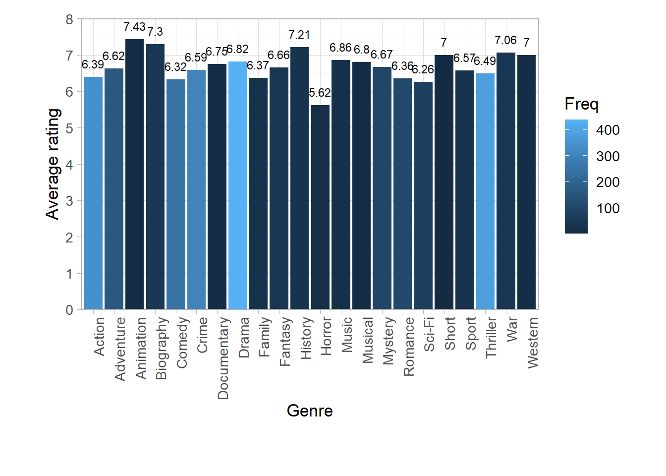

I really enjoy a great animation movie (brings out the child in me), but I hardly watch them. Horror is not my preferred genre and that shows in the number of horror movies I have seen and how I rate them.